Exploring the Formula for Stochastic Volatility Model: A Comprehensive Guide

Exploring the Formula for Stochastic Volatility Model

In the world of finance, understanding and predicting volatility is crucial for making informed investment decisions. One popular model used to analyze volatility is the Stochastic Volatility Model. This model takes into account that volatility itself is not constant, but rather fluctuates over time.

The Stochastic Volatility Model combines both random and time-varying components, making it a powerful tool for modeling and forecasting volatility. It is widely used in financial derivatives pricing, risk management, and asset allocation strategies.

Table Of Contents

This comprehensive guide aims to provide a deeper understanding of the formula for the Stochastic Volatility Model. We will explore its key elements, assumptions, and the mathematics behind it. Additionally, we will discuss the advantages and limitations of this model, as well as its practical applications in the field of finance.

By the end of this guide, readers will have a solid foundation in understanding and using the Stochastic Volatility Model. Whether you are a seasoned investor or just starting out in the world of finance, this guide will equip you with the knowledge to confidently incorporate this powerful model into your decision-making process.

Understanding the Basics of Stochastic Volatility

Stochastic volatility is a concept used in financial modeling to describe the random fluctuations in the volatility of an asset’s price over time. Unlike traditional models that assume volatility is constant, stochastic volatility models recognize that volatility can vary and follow a stochastic process.

Volatility refers to the degree of variation of an asset’s price over time. It is an important measure in financial markets as it represents the level of risk associated with an investment. Higher volatility implies a greater level of uncertainty and potential for large price movements.

In stochastic volatility models, the volatility of an asset is often modeled as a latent variable that follows a diffusion process. This means that the volatility itself is subject to random shocks and can change over time. The dynamics of the volatility process can be described by a stochastic differential equation.

The most common stochastic volatility model is the Heston model, named after Steven Heston who developed it in 1993. The Heston model assumes that the volatility follows a mean-reverting process, meaning it tends to revert back to its long-term average. This model has been widely used in the pricing and calibration of options.

Stochastic volatility models are particularly useful for capturing the skewness and kurtosis observed in financial data. Skewness refers to the asymmetry of the distribution of returns, while kurtosis measures the thickness of the distribution’s tails. These characteristics are important for accurately pricing complex derivative instruments, such as options.

Estimating stochastic volatility models can be challenging due to the nonlinearity and high dimensionality of the models. Various techniques, such as maximum likelihood estimation and Bayesian methods, have been developed to estimate the model parameters and calibrate the models to market data.

Read Also: Understanding the Distinction: ECN vs Exchange

Overall, understanding the basics of stochastic volatility is essential for financial modeling and risk management. By accounting for the stochastic nature of volatility, stochastic volatility models provide more accurate and realistic estimates of asset prices, thereby improving investment decision-making and risk assessment.

Exploring the Formula for Stochastic Volatility

Stochastic volatility is an important concept in financial modelling that aims to capture the volatility of asset prices over time. It is a well-known fact that asset prices are highly volatile and exhibit complex patterns. The stochastic volatility model provides a framework for understanding and quantifying this volatility.

In this article, we will explore the formula for stochastic volatility and its implications in financial modelling. The formula for stochastic volatility is based on the concept of a volatility process, which is assumed to follow a stochastic differential equation.

The stochastic volatility model assumes that the volatility of asset prices is not constant over time but instead evolves according to a stochastic process. This stochastic process is typically modelled as a mean-reverting process, where the volatility tends to converge to a long-term average. This is captured by the mean-reversion parameter in the formula.

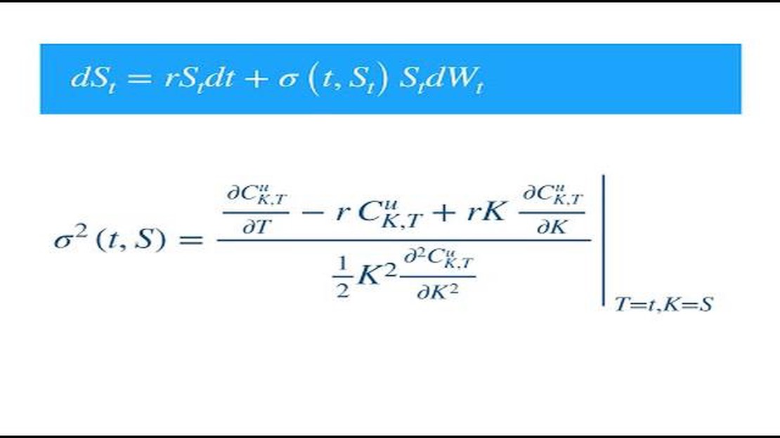
The formula for stochastic volatility can be written as:

dS(t) = μS(t)dt + σS(t)dW(t),

dσ(t) = κ(θ-σ(t))dt + ξσ(t)dZ(t),

where dS(t) is the change in the asset price at time t, μ is the drift rate of the asset price, σ is the instantaneous volatility of the asset price, dW(t) and dZ(t) are Wiener processes, κ is the mean reversion parameter, θ is the long-term average volatility, and ξ is the volatility of the volatility.

Read Also: What is the Weizmann share price forecast? Expert analysis and predictions.

The formula for stochastic volatility describes how the asset price and its volatility change over time. The first equation represents the dynamics of the asset price, where the change in the asset price is a function of its current price, drift rate, and volatility. The second equation represents the dynamics of the volatility, where the change in volatility is a function of its current value, mean reversion parameter, long-term average volatility, and volatility of the volatility.

By incorporating stochastic volatility into financial modelling, we can better capture the dynamics and variability of asset prices. This can improve the accuracy of predictions and risk management strategies. Furthermore, the formula for stochastic volatility provides a mathematical framework for exploring and understanding the underlying processes that drive asset price volatility.

In conclusion, exploring the formula for stochastic volatility is crucial for understanding and modelling the volatility of asset prices. The formula provides a mathematical representation of the dynamics of asset price and volatility, incorporating mean reversion and the volatility of the volatility. By incorporating this formula into financial models, we can improve our understanding and predictions of asset price movements.

FAQ:

What is the formula for the stochastic volatility model?

The formula for the stochastic volatility model is given by: dS(t) = µS(t)dt + σS(t)dW1(t), dσ(t) = κ(θ - σ(t))dt + ρσ(t)dW2(t), where S(t) is the asset price at time t, µ is the drift, σ is the volatility, κ is the mean reversion speed, θ is the long-term average volatility, ρ is the correlation between the asset price and volatility, and W1(t) and W2(t) are independent Brownian motions.

What are some practical applications of stochastic volatility models?

Stochastic volatility models have a wide range of applications in finance and economics. They are commonly used for pricing and hedging options, as they capture the dynamics of volatility, which is a key factor in option pricing. These models are also used for risk management and portfolio optimization, as they allow for modeling and forecasting the variability of asset returns. Additionally, stochastic volatility models can be used in macroeconomic modeling and forecasting, as they capture the time-varying nature of volatility in economic variables.

Is the stochastic volatility model a suitable choice for all types of financial data?

The stochastic volatility model may not be suitable for all types of financial data. It is primarily used for modeling assets that exhibit time-varying volatility, such as equities, currencies, and commodities. For assets with stable or constant volatility, simpler models like the Black-Scholes model may be more appropriate. However, it is important to note that the choice of model depends on the specific characteristics of the data and the objectives of the analysis.

How can stochastic volatility models be estimated?

There are several methods for estimating stochastic volatility models. One common approach is to use maximum likelihood estimation (MLE), which involves finding the set of parameter values that maximize the likelihood of observing the observed data. Another approach is Bayesian estimation, which involves specifying prior distributions for the parameters and updating them based on the observed data. Other methods include moment-based estimators, such as the method of moments or generalized method of moments, and filtering techniques, such as the Kalman filter. The choice of estimation method depends on the specific characteristics of the data and the assumptions of the model.

What are some limitations of stochastic volatility models?

Stochastic volatility models have several limitations. First, they can be computationally intensive, especially when estimating the parameters using advanced techniques like maximum likelihood estimation or Bayesian methods. Second, they may not capture all the complexities of the real world, as they assume a simplified structure for the dynamics of volatility. Third, the accuracy of the model depends on the quality and accuracy of the input data. Finally, stochastic volatility models may produce unrealistic or implausible volatility forecasts in certain situations. Despite these limitations, stochastic volatility models remain a valuable tool for understanding and modeling the dynamics of financial markets.

What is a stochastic volatility model?

A stochastic volatility model is a mathematical model used to describe the volatility of financial assets. Unlike the traditional Black-Scholes model, which assumes constant volatility, a stochastic volatility model allows for the volatility to vary over time. It takes into account the fact that the market volatility is not constant and can change unpredictably.