


Understanding the Functioning of OCO: A Comprehensive Guide
How Does OCO Work? In today’s complex and interconnected world, the need for accurate and reliable data is more important than ever. The Orbiting …
Read Article
The Generalized Linear Autoregressive Moving Average (GLARMA) model is a popular statistical model used to analyze time series data. It is an extension of the Autoregressive Moving Average (ARMA) model, which is widely used in econometrics and finance. The GLARMA model is particularly useful when dealing with non-Gaussian and non-linear data, as it allows for more flexible modeling of the relationship between the response variable and the predictor variables.
Like the ARMA model, the GLARMA model consists of two components: the autoregressive (AR) component and the moving average (MA) component. The AR component models the dependence of the response variable on its past values, while the MA component models the dependence of the response variable on its past errors. The GLARMA model also incorporates the concept of link functions, which transform the response variable to ensure that the model is appropriate for the particular type of data being analyzed.
The GLARMA model can be used to analyze a wide range of time series data, including financial data, economic data, and biomedical data. It has been widely applied in various fields, such as finance, economics, epidemiology, and environmental science. The model allows researchers to accurately model and predict the behavior of complex time series data, thereby providing valuable insights and aiding in decision-making.
In conclusion, the Generalized Linear Autoregressive Moving Average model is a powerful tool for analyzing time series data. It extends the traditional ARMA model by incorporating the concept of link functions and allowing for more flexible modeling of the relationship between the response variable and the predictor variables. The GLARMA model has been widely used in various fields, and its applications continue to grow. By understanding and utilizing this model, researchers and analysts can gain deeper insights into the dynamics of time series data and make more accurate predictions.
The Generalized Linear Autoregressive Moving Average (GLARMA) model is a statistical model used to analyze time series data. It combines elements of both autoregressive (AR) and moving average (MA) models, as well as the generalized linear model (GLM).
In the GLARMA model, the dependent variable is assumed to follow a generalized linear model, which allows for non-normal distribution and non-linear relationships between variables. This makes the GLARMA model suitable for analyzing a wide range of data types, including count data, binary data, and continuous data.
The autoregressive component of the GLARMA model considers the previous values of the dependent variable to predict the current value. This is similar to the AR model, which models the current value as a linear combination of its past values. The moving average component, on the other hand, models the error term as a linear combination of past error terms.
The GLARMA model also allows for the inclusion of exogenous variables, which can further improve the model’s predictive power. These variables can be included as additional predictors in the generalized linear model component, allowing for the analysis of their effects on the dependent variable.
Estimating the parameters of the GLARMA model typically involves maximum likelihood estimation, which involves finding the values of the parameters that maximize the likelihood of observing the given data. Once the model parameters are estimated, they can be used to make predictions and infer relationships between variables.
In summary, the GLARMA model is a flexible and powerful tool for analyzing time series data with non-normal distribution and non-linear relationships. By combining elements of autoregressive and moving average models with the generalized linear model, it can capture complex patterns and relationships in the data.
Read Also: Can I hold and use USD currency in India?
The Generalized Linear Autoregressive Moving Average (GLARMA) model is a useful tool for analyzing time series data. It combines the concepts of generalized linear models, autoregressive models, and moving average models to capture the complex relationships and patterns often found in time series data.
At its core, GLARMA consists of several key components that work together to provide a comprehensive analysis:
2. Autoregressive (AR) component: The AR component accounts for the dependency between observations within a time series. It models the current value as a linear combination of previous values, capturing the trend or seasonal patterns present in the data. 3. Moving average (MA) component: The MA component captures the short-term fluctuations or random shocks in the data. It models the current value as a linear combination of the error terms from previous observations, allowing for the consideration of random fluctuations in the time series. 4. Link function: GLARMA incorporates a link function to relate the linear predictors to the response variable. Common link functions used in GLARMA include identity, logit, and log-log, depending on the nature of the response variable.
Read Also: Step-by-step guide: How to fill out a forex card5. Error distribution: GLARMA assumes an error distribution that follows a specific probability distribution, such as Gaussian, Poisson, or binomial. The choice of the error distribution depends on the nature of the response variable and the assumptions made about the data.
Overall, the structure of GLARMA combines these key components in a flexible and powerful model that can accommodate a wide range of time series data. By combining the concepts of GLM, AR, and MA, GLARMA is able to capture both short-term fluctuations and long-term trends, making it a valuable tool for time series analysis.
The Generalized Linear Autoregressive Moving Average (GLARMA) model has a wide range of applications across various industries. Here are some of the key applications and advantages of GLARMA:

Some advantages of using GLARMA include:
In summary, GLARMA is a versatile modeling framework with numerous applications in various fields. It offers several advantages, including flexibility, the ability to handle different types of distributions, accounting for autocorrelation, and capturing moving average components. As a result, GLARMA is a valuable tool for analyzing and forecasting time series data, making predictions in financial markets, studying epidemiological dynamics, and modeling environmental phenomena.
The Generalized Linear Autoregressive Moving Average (GLARMA) model is a time series model that incorporates both autoregressive (AR) and moving average (MA) components. However, unlike traditional ARMA models, the GLARMA model is more flexible, allowing for different types of error distributions, including non-Gaussian distributions.
The GLARMA model has several benefits. First, it can capture the complex patterns and relationships present in time series data, making it a powerful tool for forecasting. Second, it allows for different types of error distributions, which is especially useful when the data does not follow a Gaussian distribution. Finally, the GLARMA model can be easily extended to include exogenous variables, further enhancing its forecasting capabilities.
The GLARMA model differs from traditional ARMA models in several ways. Firstly, while ARMA models assume Gaussian errors, the GLARMA model allows for different types of error distributions, such as the binomial or Poisson distribution. Secondly, the GLARMA model accommodates overdispersed or underdispersed data, which is common in many real-world time series. Finally, the GLARMA model can handle non-constant variances, which is important when dealing with heteroscedastic data.
Yes, the GLARMA model can be used for forecasting. The model incorporates both autoregressive and moving average components, allowing it to capture the temporal dependencies and patterns in the data. By fitting the model to historical data, it can then be used to make predictions for future time points. However, it’s important to note that the accuracy of the forecasts will depend on the quality and representativeness of the historical data, as well as the appropriateness of the GLARMA model for the specific time series.

How Does OCO Work? In today’s complex and interconnected world, the need for accurate and reliable data is more important than ever. The Orbiting …
Read Article
What is a bearish moving average? A bearish moving average is a technical indicator used in financial markets to identify a potential downtrend. It is …
Read Article
Is It Possible to Issue Stock Options Below FMV? Stock options are a common form of compensation for employees, allowing them to purchase company …
Read Article
Understanding the Net Investment Tax on Stock Options Stock options can be a lucrative form of compensation for employees, but there are some …
Read Article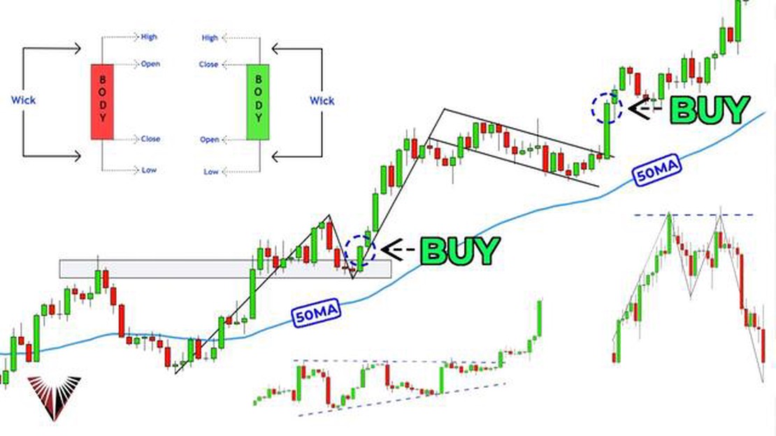
Understanding trade analysis Trade analysis is an essential tool for businesses and economists alike. It involves the examination of import and export …
Read Article
Understanding IB Rebate: A Comprehensive Guide IB rebate, also known as Introducing Broker rebate, is a form of compensation that Introducing Brokers …
Read Article


