

Is Option Trading Possible in Forex? Learn More Here
Option Trading in Forex: Everything You Need to Know Forex market is the world’s largest financial market, with billions of dollars being traded every …
Read Article
Seasonal ARIMA with Exogenous Regressors, or SARIMAX, is a powerful time series forecasting model that takes into account both seasonal patterns and external factors that influence the time series. In this comprehensive guide, we will explore the intricacies of SARIMAX and learn how to effectively use it to forecast time series data.
ARIMA, which stands for Autoregressive Integrated Moving Average, is a popular model for time series forecasting. It combines autoregression, differencing, and moving average techniques to capture the underlying patterns in the data. However, ARIMA is not suitable for time series data with seasonal patterns and external factors. This is where SARIMAX comes into play.
SARIMAX extends the capabilities of ARIMA by incorporating seasonal differencing and exogenous regressors. Seasonal differencing allows the model to capture the seasonality in the data, while exogenous regressors enable the inclusion of external factors that may influence the time series. By considering both seasonal patterns and external factors, SARIMAX is able to provide more accurate forecasts for complex time series data.
In this guide, we will cover the basics of SARIMAX, including the mathematical formulation, parameter estimation, and model diagnostics. We will also explore various techniques for selecting the optimal SARIMAX model, including grid search and information criteria. Finally, we will walk through a practical example of using SARIMAX to forecast a real-world time series dataset.
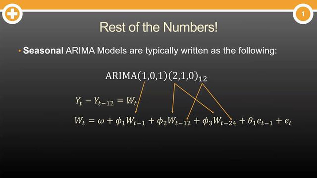
Seasonal Autoregressive Integrated Moving Average (ARIMA) is a popular time series forecasting model that takes into account both trend and seasonality in data. It is an extension of the non-seasonal ARIMA model, which is used for forecasting data without considering seasonal components.

Seasonality refers to patterns that repeat at regular intervals, such as daily, weekly, or monthly cycles. These patterns can have a significant impact on the data and can be observed in various fields, including economics, finance, and meteorology. In order to effectively forecast time series data with seasonal patterns, it is necessary to use a model that captures both the trend and the seasonality.
The Seasonal ARIMA model accomplishes this by incorporating additional terms that account for the seasonal component of the data. It includes three main components:
By combining these components, the Seasonal ARIMA model is able to capture and forecast both the trend and the seasonal patterns in the data. It provides a powerful tool for analyzing and predicting time series data with seasonal fluctuations.
Seasonal ARIMA (AutoRegressive Integrated Moving Average) is a powerful time series forecasting model that combines the concepts of ARIMA with the ability to account for seasonality in the data. Seasonal ARIMA is widely used in various fields, including finance, economics, and the energy sector.
In a nutshell, the Seasonal ARIMA model takes into account both the non-seasonal and seasonal components of a time series in order to make accurate forecasts. It achieves this by incorporating three main components:
Read Also: Who owns UBS? Discover the major shareholders of UBS Group AG
In addition to these components, Seasonal ARIMA also incorporates the concept of seasonality through the use of seasonal differencing. Seasonal differencing involves taking the difference between observations that are spaced a specific number of time units apart (e.g., differences between observations in the same month of different years). This helps remove the seasonal patterns from the time series.
The parameters of a Seasonal ARIMA model are typically determined through a process called model selection. This involves selecting the values of the AR, MA, and seasonal components that best fit the data. This process typically includes assessing the autocorrelation and partial autocorrelation functions of the time series to determine the appropriate lag orders, as well as selecting the appropriate differencing levels to achieve stationarity.
Read Also: Understanding Stock Options for New Hires: A Comprehensive Guide
Once the parameters are determined, the Seasonal ARIMA model can be used to make forecasts for future time periods. These forecasts take into account both the non-seasonal and seasonal components, making them particularly useful for capturing and predicting seasonal patterns in the data.
In conclusion, Seasonal ARIMA is a versatile and powerful model for forecasting time series data with seasonality. By incorporating the concepts of ARIMA and seasonal differencing, it is able to capture and predict both the non-seasonal and seasonal components of a time series, making it an invaluable tool in many fields.
ARIMA models are statistical models that are used to analyze and forecast time series data. They are a combination of autoregressive (AR), moving average (MA), and differencing (I) components.
Exogenous regressors can be incorporated into ARIMA models by adding them as additional explanatory variables in the model. This allows the model to account for the effect of these regressors on the time series being analyzed.
The purpose of using seasonal ARIMA models is to capture and model the seasonal patterns that may be present in the time series data. These models are useful when the data shows repetitive patterns over fixed time intervals.

The order of the ARIMA model can be determined by analyzing the autocorrelation function (ACF) and partial autocorrelation function (PACF) plots of the time series data. These plots can help identify the appropriate values for the AR, MA, and differencing components of the model.
Yes, exogenous regressors can be used in both the autoregressive (AR) and moving average (MA) components of the ARIMA model. This allows the model to account for the influence of these regressors on both the past values and the prediction errors of the time series.
The purpose of using exogenous regressors in seasonal ARIMA is to incorporate external variables or factors that may have an impact on the time series being analyzed. These exogenous regressors can help improve the accuracy of the forecast by capturing additional information that is not present in the time series data alone.

Option Trading in Forex: Everything You Need to Know Forex market is the world’s largest financial market, with billions of dollars being traded every …
Read Article
The speed of the largest tornado in history Tornadoes are some of the most destructive natural phenomena on Earth. Their powerful winds can cause …
Read Article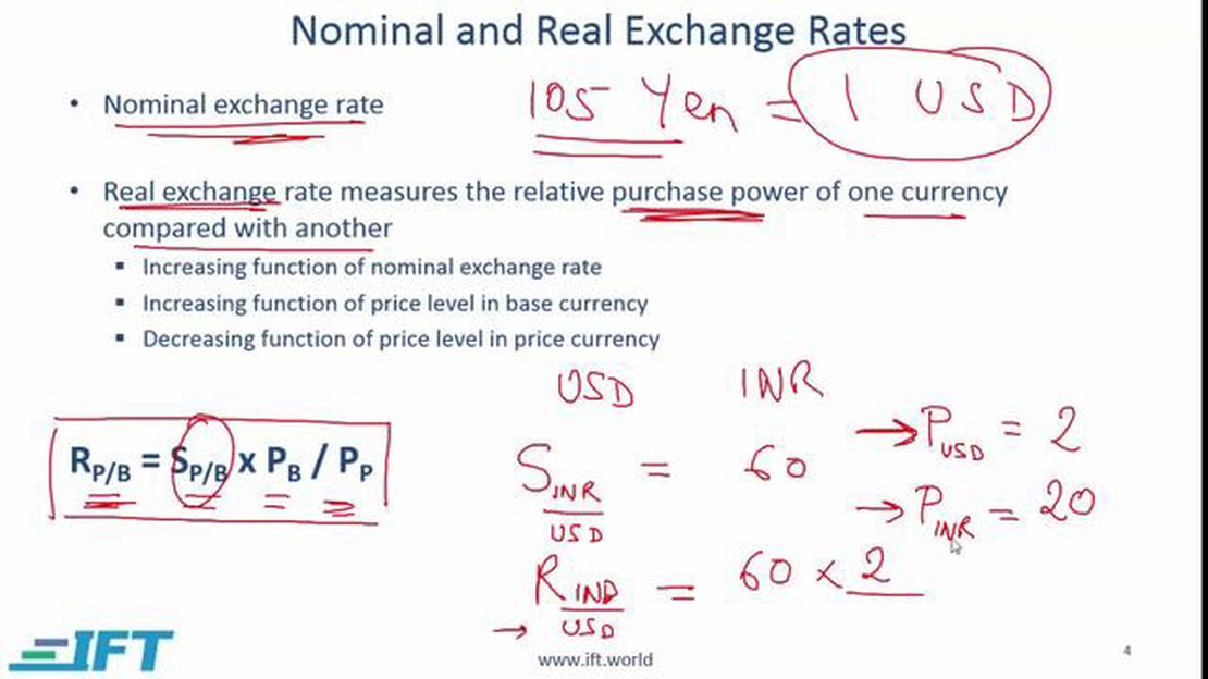
Understanding the distinction between XOF and CFA currencies Both XOF and CFA are currencies used in various African countries, but they are not the …
Read Article
Is Trading Options Similar to Gambling? When it comes to trading options, there are often misconceptions that it is similar to gambling. However, this …
Read Article
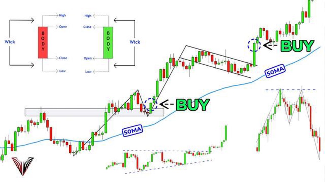
Indicators for Momentum Trading: A Comprehensive Guide In the world of trading, there are many strategies that traders employ to try and capitalize on …
Read Article
4h Time Frame Strategy: Everything You Need to Know In the world of trading, time frames play a crucial role in determining the success of a strategy. …
Read Article


