

Understanding the Hull Moving Average Indicator in MT4: A Comprehensive Guide
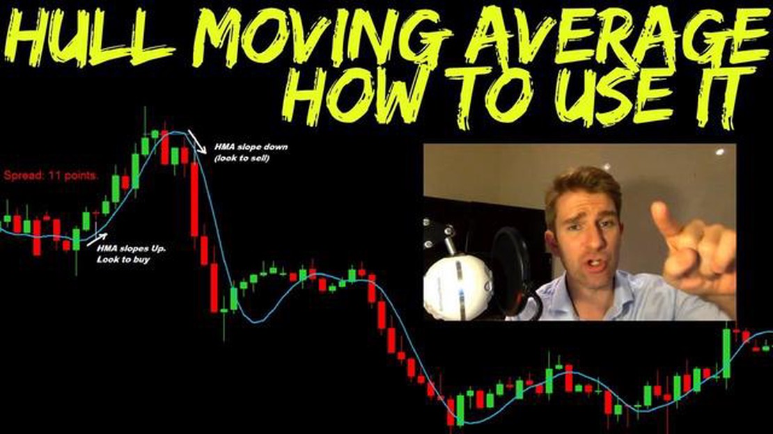
What is the hull moving average indicator in MT4? When it comes to technical analysis in the forex market, traders have a wide range of indicators at …
Read Article
In the world of time series analysis, the ARIMA model is a popular choice for modeling and forecasting data. ARIMA stands for AutoRegressive Integrated Moving Average, and it combines the concepts of autoregression, differencing, and moving average to capture the complex patterns in time series data. In this comprehensive guide, we will focus specifically on the moving average component of the ARIMA model.
The moving average model, also known as the MA model, is a key component of ARIMA. It helps to capture the random components or noise present in the time series data. The MA model is based on the idea that the value of the time series at any given point is a linear combination of past error terms, also known as residuals.
The moving average model is defined by two main parameters – the order of differencing (d) and the order of the moving average (q). The order of differencing determines the number of times the time series needs to be differenced to make it stationary, while the order of the moving average determines the number of error terms to be included in the model. By understanding and correctly specifying these parameters, we can build an accurate and effective MA model to analyze and forecast time series data.
In this guide, we will cover the concept of the moving average model in detail, including its mathematical formulation, interpretation of parameters, and steps to build and evaluate the model. We will also discuss practical examples and case studies to illustrate its application in real-world scenarios. By the end of this guide, you will have a comprehensive understanding of the moving average model in ARIMA and be equipped with the knowledge to apply it to your own time series data.
In the context of ARIMA, the Moving Average (MA) model is a key component that helps in analyzing and forecasting time series data. Its main focus is on the dependence between an observation and a residual error from a moving average process.
The MA model consists of three main components:

The MA model can be represented as:
Xt = μ + εt + θ1εt-1 + θ2εt-2 + … + θqεt-q
Here, Xt represents the time series at time t, μ is the constant, εt is the random error at time t, θi represents the coefficients of the MA model, and q represents the order of the MA model.
Read Also: Can You Trade Forex (FX) in China? Exploring China's Forex Market
The MA model captures short-term dependencies and fluctuations in the time series by modeling the relationship between the observation and the residual errors. It is particularly useful in cases where the time series exhibits random or unpredictable behavior.
By analyzing the components of the MA model and estimating the values of the parameters, we can gain insights into the underlying patterns and trends in the time series. This, in turn, allows us to make accurate forecasts and predictions based on the observed data.
The moving average (MA) model is an essential component of the autoregressive integrated moving average (ARIMA) model. It is used to understand and predict the behavior of time series data. In this section, we will explore how to apply the moving average model in the ARIMA framework.
In the ARIMA model, the moving average component is responsible for capturing the short-term fluctuations in the data. It helps to smooth out the noise and identify any underlying patterns or trends. To apply the moving average model in ARIMA, we need to understand how to select the appropriate order of the model.
The order of the moving average model is denoted as MA(q), where “q” represents the number of lagged moving average terms to include in the model. The lagged moving average terms are the weighted average of the past error terms. It is important to choose an appropriate value for “q” to accurately capture the short-term dynamics of the data.
There are several ways to determine the order of the moving average model. One common approach is to use the autocorrelation function (ACF) and partial autocorrelation function (PACF) plots. The ACF plot helps to identify the potential order of the moving average component, while the PACF plot helps to determine the order of the autoregressive component.
Read Also: Understanding the Significance of Bollinger Bands in Technical Analysis
Another approach is to use information criteria such as the Akaike information criterion (AIC) and Bayesian information criterion (BIC). These criteria provide a balance between model complexity and goodness of fit, allowing us to select the best order for the moving average model.
Once we have determined the order of the moving average model, we can estimate the model parameters using techniques like maximum likelihood estimation. The estimate of the model parameters allows us to make predictions and forecast future values based on the observed data.
Overall, the moving average model is a powerful tool for analyzing time series data. By applying it within the ARIMA framework, we can accurately capture the short-term dynamics and make meaningful predictions. Understanding how to select the appropriate order and estimate the model parameters is crucial for getting reliable results.

The moving average model in ARIMA is a statistical technique used to forecast future values in a time series based on the average of the previous values in the series. It is a component of the ARIMA model, which stands for Autoregressive Integrated Moving Average.
The moving average model differs from other models, such as the autoregressive model, in that it takes into account the average of the previous values in the series rather than just the previous values themselves. This helps to smooth out any irregularities or fluctuations in the data and provides a more accurate forecast.
There are several advantages of using the moving average model in ARIMA. Firstly, it helps to eliminate any short-term fluctuations in the data, providing a more stable and accurate forecast. Secondly, it is a relatively simple model to understand and implement. Lastly, it can be used to forecast future values in a time series with a high level of accuracy.
Yes, the moving average model in ARIMA can be used for any type of time series data, as long as the data exhibits some form of trend or seasonality. However, it is important to note that the moving average model may not be suitable for all types of data, and other models, such as the autoregressive model, may need to be used in conjunction with it to provide a more accurate forecast.

What is the hull moving average indicator in MT4? When it comes to technical analysis in the forex market, traders have a wide range of indicators at …
Read Article
Exchange foreign currency at SBI If you are planning to travel abroad or have recently returned from a foreign trip, you may be wondering if you can …
Read Article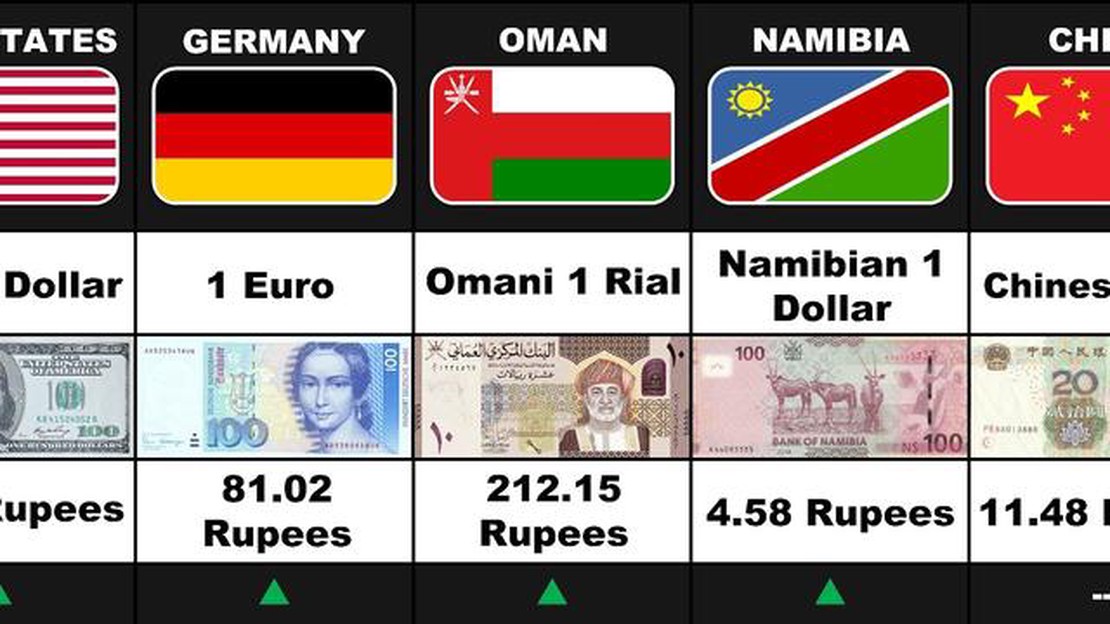
The Highest Exchange Rate with Indian Rupee Are you planning a trip to India and want to get the best exchange rate for your money? Look no further! …
Read Article
Learn the 3 Essential Chords to Play Any Song Have you ever dreamed of playing your favorite songs on the guitar but feel intimidated by all those …
Read Article
Understanding Dividends and Stock Options When it comes to investing in the stock market, many investors are interested in the potential benefits of …
Read Article
Challenges in Pricing Options: Exploring the Complexity Option pricing is a crucial aspect of financial markets. It enables investors to determine the …
Read Article


