Is MA(1) stationary? Explanation and Examples

Is Ma 1 stationary?

Stationarity is a fundamental concept in time series analysis. It refers to the statistical properties of a process remaining constant over time. One common model used in time series analysis is the Moving Average (MA) model. The MA model is characterized by the presence of a finite number of lagged values of the error term in the regression equation.

Table Of Contents

But is MA(1) stationary? In this article, we will explore the stationarity of MA(1) and provide examples to support our findings.

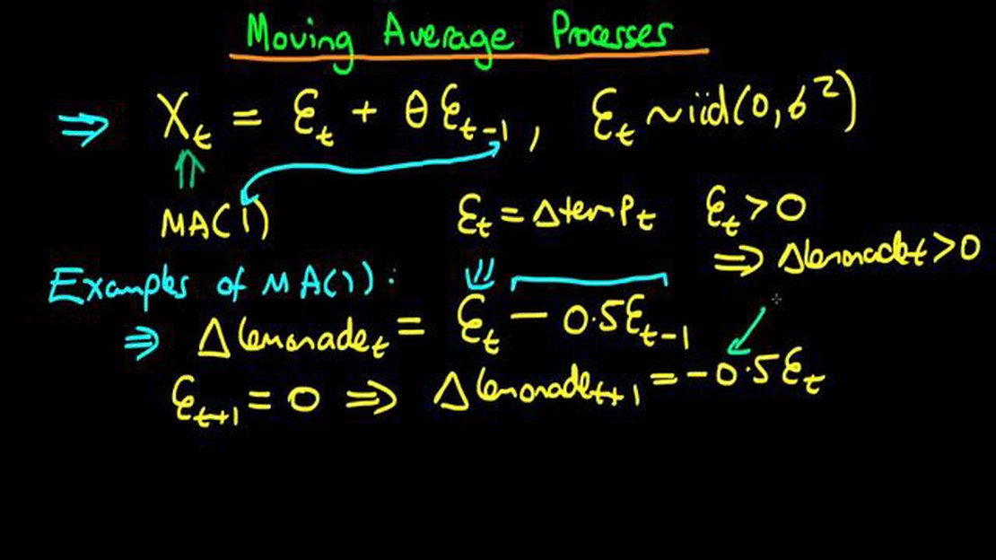
To assess the stationarity of MA(1), we first need to understand the autoregressive (AR) and moving average (MA) processes. An MA(1) process has a moving average term that depends on the error term from the previous period. It can be expressed as Xt = μ + εt + θεt-1, where Xt is the time series, μ is the mean, εt is the error term at time t, and θ is the coefficient for the moving average term.

When examining the stationarity of MA(1), we focus on the condition that the absolute value of θ is less than 1. If |θ| < 1, then the process is stationary. However, if |θ| ≥ 1, the process is non-stationary. This is because a value of θ ≥ 1 implies the moving average term has a long-term influence, which can cause the process to drift over time.

Example:

Let’s consider an example to illustrate the stationarity of MA(1). Suppose we have an MA(1) process defined as Xt = εt + 0.6εt-1. If we choose a value of θ = 0.6, which satisfies |θ| < 1, then the process is stationary. This means that the statistical properties of the process, such as mean and variance, remain constant over time. On the other hand, if we were to choose a value of θ = 1.2, which satisfies |θ| ≥ 1, then the process would be non-stationary, as the moving average term has a long-term influence that can cause the process to drift away from its mean.

What is Stationarity in Time Series?

Stationarity is an important concept in time series analysis. It refers to the statistical properties of a time series that remain constant over time. A stationary time series has a constant mean, a constant variance, and an autocovariance that only depends on the time lag.

In simpler terms, a stationary time series can be described as one that does not exhibit any trend or seasonality. The mean and variance of the series remain constant, and the correlation between observations at different time points remains the same.

There are different types of stationarity, including weak stationarity, strict stationarity, and ergodic stationarity. Weak stationarity refers to a series with a constant mean, variance, and autocovariance, while strict stationarity refers to a series where the joint distribution of any set of observations is invariant to shifts in time. Ergodic stationarity combines the properties of weak and strict stationarity, implying that sample means are representative of population means.

Stationarity is an important assumption in many time series models and techniques. It allows for the use of statistical methods that rely on the constancy of key properties, such as the autocorrelation function. Non-stationary series can lead to biased and inconsistent results in modeling and forecasting.

Identifying whether a time series is stationary or not is a crucial step in time series analysis. This can be done through visual inspection of plots, such as time series plots and autocorrelation plots, and through statistical tests, such as the Augmented Dickey-Fuller test.

Type of Stationarity	Description
Weak Stationarity	A series with a constant mean, variance, and autocovariance.
Strict Stationarity	A series where the joint distribution of any set of observations is invariant to shifts in time.
Ergodic Stationarity	A series that combines the properties of weak and strict stationarity, implying that sample means are representative of population means.

Meaning of MA(1) Model in Time Series

The MA(1) model, also known as the Moving Average model of order 1, is a type of time series model used to predict future values based on the previous error terms. In this model, the current value of the time series is a linear combination of the current error term and the previous error term. The MA(1) model is defined by the equation:

Xt = μ + εt + θ1εt-1

where Xt represents the current value of the time series, μ is the mean of the time series, εt is the current error term, εt-1 is the previous error term, and θ1 is the parameter that determines the weight of the previous error term.

Read Also: How to Prevent Slippage in Forex Trading: Tips and Strategies

The MA(1) model is often used to analyze time series data that exhibits a random and unpredictable pattern, as it allows for the inclusion of the randomness in the prediction process. By including the previous error term in the model, the MA(1) model captures the short-term dependencies and helps in forecasting future values.

The parameter θ1 plays a crucial role in the MA(1) model. If θ1 is positive, it suggests that there is positive autocorrelation between the current error term and the previous error term, meaning that an increase in the current error term would result in an increase in the previous error term. Conversely, if θ1 is negative, it indicates negative autocorrelation.

Read Also: What about Forex? Everything You Need to Know

Overall, the MA(1) model is a useful tool in time series analysis for predicting future values based on the previous error terms. It helps in understanding the short-term dependencies and random patterns in the data, providing valuable insights for forecasting and decision making.

Testing Stationarity of MA(1) Model

Stationarity is an important property of a time series model. A stationary time series has constant mean and variance over time, and its autocovariance function does not depend on the time at which it is computed.

Testing the stationarity of an MA(1) model involves verifying if the model satisfies these conditions. One common method for testing stationarity is the Augmented Dickey-Fuller (ADF) test.

The ADF test is a statistical test that determines the presence of unit roots in the time series. A unit root is an indicator of non-stationarity. The ADF test null hypothesis assumes the presence of unit roots in the time series, while the alternative hypothesis assumes stationarity.

To perform the ADF test on an MA(1) model, we can start by estimating the parameters of the model using maximum likelihood estimation (MLE). Once the parameters are estimated, we can calculate the residuals of the model and perform the ADF test on these residuals.

If the p-value of the ADF test is less than a chosen significance level (e.g., 0.05), we reject the null hypothesis of non-stationarity and conclude that the MA(1) model is stationary. If the p-value is greater than the significance level, we fail to reject the null hypothesis and conclude that the MA(1) model is non-stationary.

It’s important to note that the ADF test assumes that the residuals are normally distributed and independent. If these assumptions are violated, alternative tests such as the Kwiatkowski-Phillips-Schmidt-Shin (KPSS) test can be used.

Overall, testing the stationarity of an MA(1) model involves estimating the model parameters, calculating the residuals, and performing the ADF test on these residuals. By analyzing the p-value of the ADF test, we can determine if the MA(1) model is stationary or not.

FAQ:

What is a MA(1) model?

A MA(1) (Moving Average 1) model is a type of time series model that includes the current value of the time series and one lagged value in its formulation.

What does it mean for a MA(1) model to be stationary?

A stationary MA(1) model means that its properties do not change over time. In other words, the mean and variance of the process remain constant throughout the time series.

How can we determine if a MA(1) model is stationary?

To determine if a MA(1) model is stationary, we need to check if the model satisfies certain conditions. These conditions include a constant mean, constant variance, and no autocorrelation.

Can you provide an example of a stationary MA(1) model?

Sure! An example of a stationary MA(1) model is given by: Xt = 0.5Zt-1 + Zt, where Xt is the current value of the time series, Zt is a white noise process with mean zero and variance sigma^2.

What are the implications if a MA(1) model is not stationary?

If a MA(1) model is not stationary, it means that its properties change over time. This can lead to difficulties in analyzing and forecasting the time series data, as the mean, variance, and autocorrelation may not remain constant.